3.7 - Unemployment
Definition and measurement of unemployment
Unemployment occurs when people who are capable of working are unable to find suitable jobs despite actively seeking them.
Key concepts in defining unemployment
An individual counts as unemployed if they are actively searching for work but cannot secure a position. The labour force consists of everyone who is either employed or unemployed. The population of working age, usually those between 15 and 64 years old, includes people outside the labour force.
Formula for unemployment rate
Where:
- Number of unemployed = People actively looking for work but without jobs
- Labour force = Total of employed and unemployed individuals
Difficulties in measuring unemployment
Official unemployment figures provide valuable insights but often fail to capture the full picture due to various limitations.
Reasons official statistics may underestimate unemployment
- Discouraged workers - Individuals who have given up searching for jobs after prolonged failure.
- Underemployed people - Those working fewer hours than desired or in positions that do not utilise their skills.
- Hidden unemployment - A term that covers both discouraged workers and the underemployed.
Reasons official statistics may overestimate unemployment
- Some people hide their actual employment to continue claiming benefits or to evade taxes.
- Individuals involved in illegal work may claim to be unemployed.
Limitations in revealing disparities
Unemployment data often overlook variations across different groups.
Additional measures of unemployment:
- Youth unemployment - Focuses on those aged 15-24.
- Long-term unemployment rate - Measures the percentage of the labour force unemployed for 12 months or more.
Types and causes of unemployment
Unemployment can be categorised into different types, each with specific causes.
Seasonal unemployment
Seasonal unemployment arises from predictable fluctuations in labour demand. Official statistics are often adjusted seasonally to reveal underlying trends.
Frictional unemployment
Frictional unemployment occurs when workers are temporarily between jobs. This type is usually short-term and largely unavoidable. It can be reduced by improving access to job vacancy information.
Cyclical unemployment
Cyclical unemployment is linked to economic downturns, where falling aggregate demand leads to reduced business activity and job losses. During recessions, firms cut staff because wages do not easily decrease (known as downward wage stickiness). Governments can address this through demand-side policies.
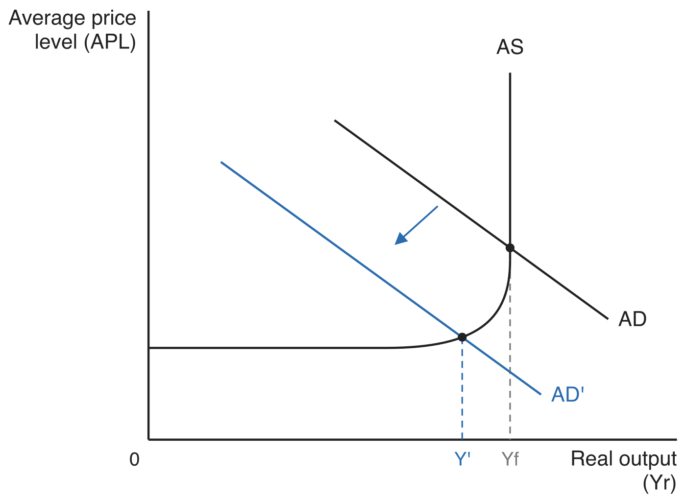
The diagram below shows this in the Keynesian model, with real output (Yr) on the horizontal axis and the average price level (APL) on the vertical axis. The economy starts at the full employment level of output Yf, where aggregate demand AD meets aggregate supply AS. When aggregate demand falls to AD', output settles at Y' instead, and the average price level falls only a little because AS is almost flat below full employment. The gap Y'Yf is the deflationary gap: the further output sits below Yf, the more workers firms lay off, so the greater the cyclical unemployment.
Structural unemployment
Structural unemployment persists even in recovering economies due to mismatches between available jobs and workers' skills or locations.
Types of structural unemployment:
- Skills mismatch - Job openings exist, but unemployed individuals lack the necessary qualifications, often due to technological changes.
- Geographic mismatch - Jobs are available in one region, but unemployed workers live elsewhere.
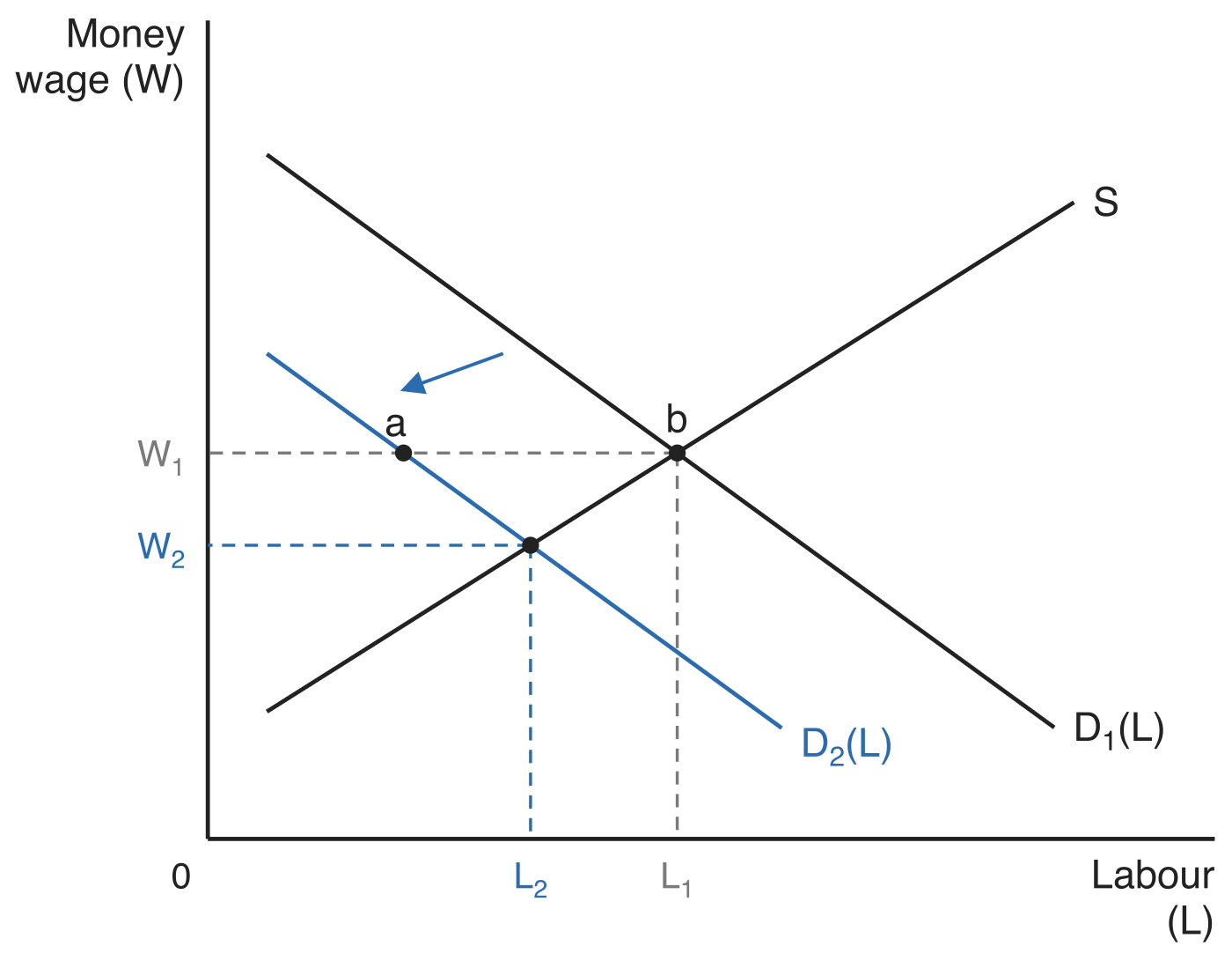
Structural unemployment usually starts with a fall in demand for one industry's labour, for example when cheaper foreign competitors take over its export markets. The diagram below shows the market for that industry's specialised workers, with the money wage (W) on the vertical axis and labour (L) on the horizontal axis. Labour demand falls from D1(L) to D2(L). At the original wage W1 firms want only the number of workers at point a, while point b on the labour supply curve S is the number still willing to work at that wage, so the distance ab is the unemployment that results. Even if the wage does fall to W2, employment settles at L2 rather than L1, so the workers between L2 and L1 lose their jobs. Because money wages are sticky downwards they tend to stay at or near W1, which leaves unemployment higher still, and those workers stay unemployed until they gain the skills the vacancies ask for or move to where the jobs are.
Labour market rigidities:
- Minimum wage laws.
- High non-wage costs.
- Strong trade unions negotiating elevated wages.
- Strict job protection laws.
- Generous unemployment benefits that reduce the incentive to accept available jobs.
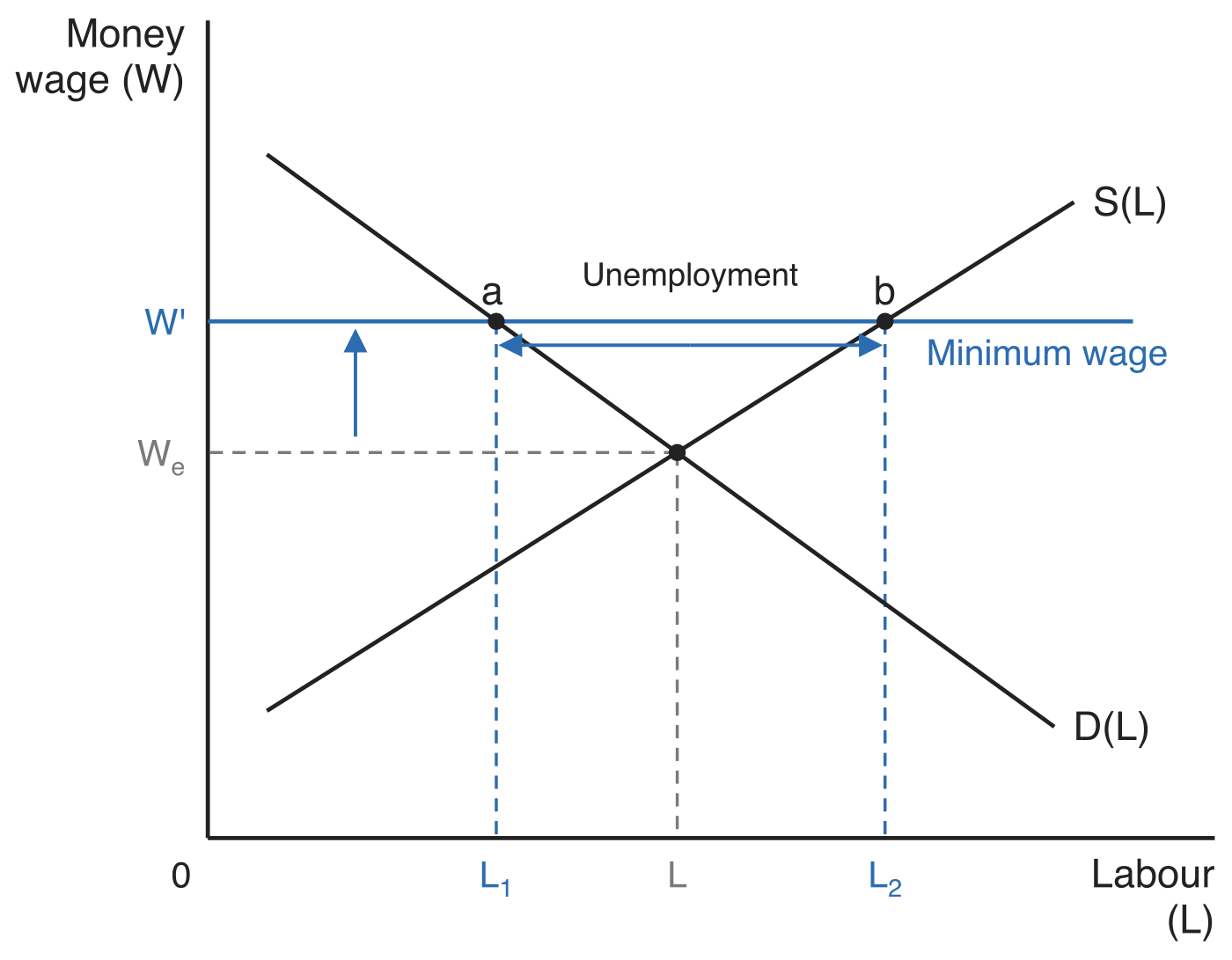
A minimum wage shows how a rigidity of this kind creates unemployment. In the diagram below the minimum wage W' is set above the market equilibrium wage, where labour demand D(L) and labour supply S(L) cross at L. At W' firms want only L1 workers, while L2 workers offer their labour, so there is an excess supply of labour: the distance ab, from a on D(L) to b on S(L). Those L1L2 workers make up the resulting unemployment, and because the wage cannot fall back to We the market has no way of clearing.
The natural rate of unemployment
The natural rate of unemployment (NRU) represents the baseline level of unemployment that exists even in a balanced economy, excluding cyclical factors.
Components of the natural rate of unemployment
The natural rate includes seasonal, frictional, and structural unemployment. It represents the equilibrium point where labour supply and demand balance. Not all individuals in this category choose to be unemployed; many struggle to find suitable roles.
The labour market equilibrium model
In this model, curves illustrate how wages affect employment levels:
- Labour demand curve (LD) - Shows the number of workers firms want to hire at various wage rates. A higher real wage means firms hire fewer workers, so it slopes downwards.
- Labour force curve (LF) - Indicates how many people are willing to enter the job market at different wages. A higher real wage draws more people in, so it slopes upwards.
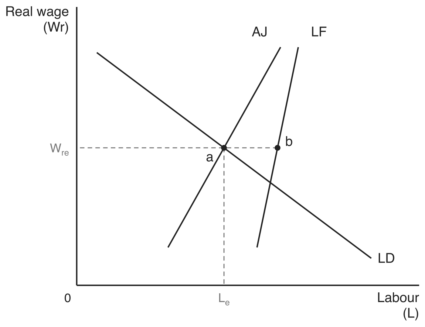
- Accept jobs curve (AJ) - Represents the number of people who will accept job offers at each wage level. It lies to the left of LF, because at any wage some of the labour force turn offers down, and the two curves converge as the real wage rises further above unemployment benefits.
The diagram below puts the three curves together, with the real wage (Wr) on the vertical axis and labour (L) on the horizontal axis. The market is in equilibrium at the real wage Wre, where the number of workers firms want to hire equals the number willing to accept a job offer, Le. The labour force at that wage is larger than the number accepting jobs, and the horizontal distance ab between AJ and LF is the natural rate of unemployment. If policymakers cut unemployment benefits, AJ shifts right, ab narrows and the NRU falls.