4.23 - Marshall-Lerner Condition & J-curve Effect

Trade effects of devaluation or depreciation

Currency devaluation or a sharp depreciation reduces the foreign price of a country's exports while increasing the domestic price of its imports. This change can make exports more attractive to overseas buyers and imports less appealing to domestic consumers, potentially leading to higher export revenues and lower import spending.

How devaluation impacts trade

• Exports - Become cheaper in foreign currencies, which can boost demand abroad if buyers respond to the lower prices. This may increase overall export revenues, especially if the quantity sold rises enough to offset the price drop.
• Imports - Become more expensive in the domestic currency, even if their foreign price stays the same. This can reduce demand for imported goods, leading to lower import expenditures as consumers and businesses switch to local alternatives.

The overall effect on a country's trade balance depends on the price elasticity of demand (PED) for both exports and imports. PED measures how much the quantity demanded changes in response to a price change.

The Marshall-Lerner condition and trade deficits

The Marshall-Lerner condition determines whether a currency devaluation or depreciation will improve a trade deficit, where import spending exceeds export revenues. It focuses on the combined responsiveness of demand for exports and imports to price changes.

Requirements of the Marshall-Lerner condition

The condition states that devaluation will reduce a trade deficit if the PED for exports and the PED for imports, taken as absolute values, sum to more than 1:

$$|{\text{PED}}_{\text{X}}|+|{\text{PED}}_{\text{M}}|>1$$

Where:

• PED_X = Price elasticity of demand for exports

• PED_M = Price elasticity of demand for imports

• If PED_X exceeds 1 in absolute terms, export revenues rise because the percentage increase in quantity demanded exceeds the percentage fall in price.

• If PED_M exceeds 1 in absolute terms, import expenditures fall because the percentage decrease in quantity demanded exceeds the percentage rise in price.

• When the sum exceeds 1, the positive effects on exports and imports together improve the trade balance.

Worked example - The Marshall-Lerner condition

A country has a trade deficit. The PED for its exports is 0.5, and the PED for its imports is 0.7. Following a currency depreciation, determine if the trade deficit will improve according to the Marshall-Lerner condition.

Step 1: Identify the values

• PED_X = 0.5
• PED_M = 0.7

Step 2: Apply the Marshall-Lerner condition

$${\text{PED}}_{\text{X}}+{\text{PED}}_{\text{M}}=0.5+0.7=1.2$$

Step 3: Check the condition

1.2 > 1, so the condition is satisfied.

Step 4: Interpretation

The trade deficit is expected to improve because the combined elasticities are elastic enough for export revenues to rise and import expenditures to fall sufficiently.

Reasons for low short-term price elasticities

The Marshall-Lerner condition is often not met immediately after devaluation because PED for exports and imports tends to be low (inelastic) in the short term. Over time, as adjustments occur, elasticities increase, and the condition may become satisfied.

Factors causing low short-term PEDs

• Limited consumer awareness - Buyers may not immediately notice or react to new prices, delaying changes in purchasing behaviour.
• Time to adjust habits - Consumers and businesses need time to alter their buying patterns, such as finding alternative suppliers or products.
• Existing contracts - Firms may be locked into long-term agreements at old prices, preventing quick switches.
• Stockpiled inventories - Businesses might use up existing stocks of imports before ordering new ones at higher prices, postponing the impact on demand.

J-curve effect of devaluation or appreciation

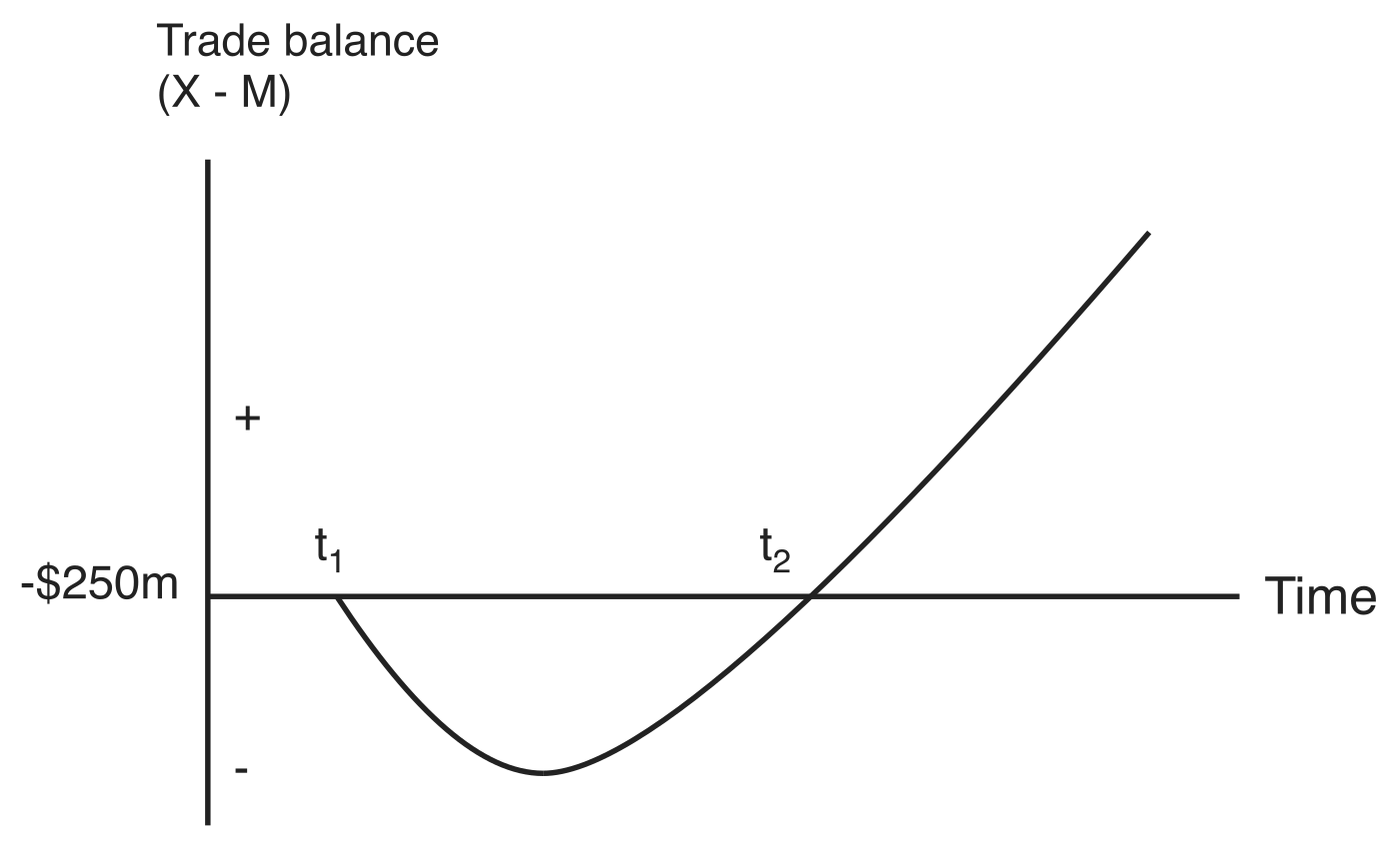
The J-curve effect describes how a trade deficit typically worsens in the short term after devaluation before eventually improving, forming a J-shape when plotted over time. This occurs because PEDs are initially low, so the Marshall-Lerner condition is not met right away.

The diagram below shows this. Time runs along the horizontal axis and the trade balance in goods and services (X - M) is measured up the vertical axis, so moving up the axis (+) means an improving balance and moving down (-) a worsening one. Take a country running a deficit of -$250m that devalues at time t1. The balance falls further below -$250m as the deficit widens, bottoms out, and only returns to -$250m at time t2, the point at which the Marshall-Lerner condition is finally satisfied. After t2 the deficit carries on shrinking.

Features of the J-curve effect

• Initial worsening - Right after devaluation at t1, import prices rise quickly, increasing import costs, while export demand grows slowly due to inelastic PEDs. This enlarges the trade deficit temporarily, and is the falling stretch of the curve.
• Later improvement - As time passes, PEDs become more elastic, satisfying the Marshall-Lerner condition. Export revenues then rise, and import spending falls, reducing the deficit, so the curve climbs back to -$250m at t2 and keeps rising after it.
• Inverted J-curve - After currency appreciation (revaluation), a trade surplus initially grows larger as imports become cheaper and exports more expensive, but it later diminishes as demand adjusts. Plotted the same way, that path traces an upside-down J.