17.6 - Rate Equations
- 1What a rate equation is
- 2How orders of reaction relate to reactant concentrations
- 3Calculations involving the rate equation
- 4Graphical representations of zero, first and second order reactions
Rate equations relate reaction rate to reactant concentrations
A rate equation is a mathematical expression that shows how the rate of a chemical reaction depends on the concentrations of the reactants.
For a general reaction: A + B ➔ C + D
The rate equation takes the form:
Rate = k[A]m[B]n
Where:
- Rate is the reaction rate (mol dm-3 s-1).
- k is the rate constant.
- [A] and [B] are the concentrations of reactants A and B (mol dm-3).
- m and n are the orders of reaction with respect to A and B.
Reaction orders show how reactant concentrations affect the rate
The values of m and n in the rate equation are the reaction orders with respect to each reactant.
They indicate how changing the concentration of a reactant influences the reaction rate.
- Zero order (m or n = 0) - The rate is independent of the reactant concentration. Doubling or tripling the concentration has no effect on the rate. [A]0 = 1, so zero order terms are often written without the concentration term.
- First order (m or n = 1) - The rate is directly proportional to the reactant concentration. Doubling the concentration doubles the rate, tripling the concentration triples the rate.
- Second order (m or n = 2) - The rate is proportional to the square of the reactant concentration. Doubling the concentration quadruples the rate (22 = 4), tripling the concentration increases the rate ninefold (32 = 9).
The overall order of the reaction is the sum of m and n.
Importantly, reaction orders can only be determined experimentally, not from balanced chemical equations.
Determining reaction orders from experimental data
To find the order of a reactant, we measure the initial reaction rate while varying the concentration of that reactant and keeping all other concentrations constant.
Worked example 1 - Determining the rate equation
Consider the reaction below, carried out at a constant temperature.
2NO(g) + O2(g) ➔ 2NO2(g)
| Experiment | [NO] (mol dm-3) | [O_2_] (mol dm-3) | Initial rate (mol dm-3 s-1) |
|---|---|---|---|
| 1 | 0.05 | 0.05 | 0.020 |
| 2 | 0.10 | 0.05 | 0.080 |
| 3 | 0.05 | 0.10 | 0.040 |
Determine the rate equation for this reaction.
Step 1: Analyse NO concentration change
Between experiments 1 and 2, the concentration of [NO] doubles while [O2] remains constant, and the rate quadruples. This suggests the reaction is second order with respect to [NO].
Step 2: Analyse O2 concentration change
Between experiments 1 and 3, doubling the concentration of [O2] while keeping [NO] constant doubles the rate, indicating first-order dependence on [O2].
Step 3: Write the rate equation
rate = k[NO]2[O2]
Worked example 2 - Calculating the rate constant
Using the same reaction and data from the previous worked example 1, calculate the rate constant (k), including its units. Give your answer to 3 significant figures.
Step 1: Rearrange rate equation
First, rearrange the rate equation to solve for k.
$\text{k }=\frac{\text{rate}}{\text{[NO]}^2[\text{O}_2]}$
Step 2: Substitution and correct evaluation
Substitute values from one of the experiments into the equation to find k. For example, substituting values from experiment 1:
$\text{k }=\frac{\text{0.020}}{(0.05)^2 \times 0.05} =160$
Step 3: Determine the units
Given that the rate is expressed in mol dm-3 s-1 and the concentration cubed in (mol dm-3)3, solving for k in the equation results in units of mol-2 dm6 s-1.
Therefore the rate constant for the reaction above is 160 mol-2 dm6 s-1.
Graphical representation of zero, first and second order reactions
The order of a reaction with respect to a reactant can be visualized using two types of plots:
- Rate-concentration curves - These plots show the reaction rate ($\nu$) against reactant concentration [X] for a series of experiments. The shape of the curve indicates the order:
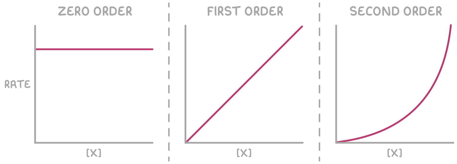
| Reaction order | Rate equation | Curve | k |
|---|---|---|---|
| zero | v = k | horizontal line | y-axis intercept |
| first | v = k[X] | straight line through the origin | gradient |
| second | v = k[X]^2^ | parabola | init at [X] = 1 mol dm^-3^ |
2. Concentration-time curves - These plots show reactant concentration against time for a single experiment. The shape of the curve depends on the order:
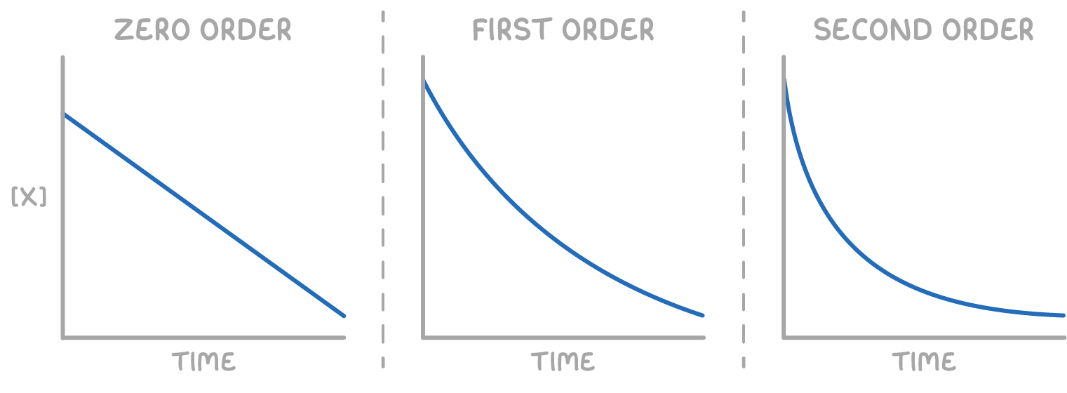
First and second order concentration-time plots can be difficult to distinguish visually. To identify the order, the data can be replotted to give a straight line graph whose gradient relates to k:
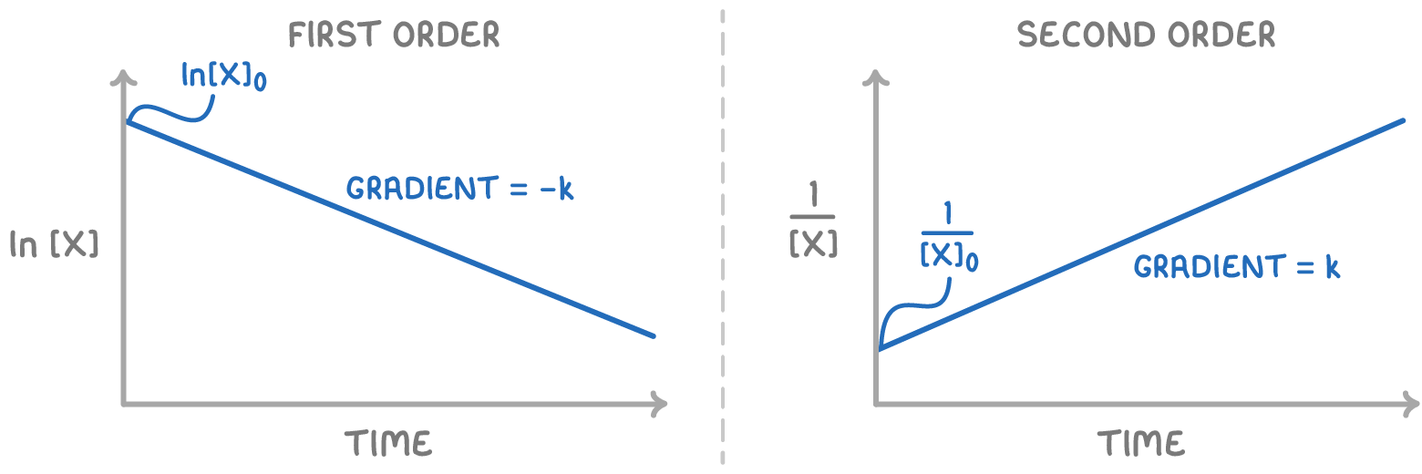
| Reaction order | y-axis | x-axis | Gradient | y-intercept |
|---|---|---|---|---|
| Zero | [X] | time | [X]0 | |
| First | ln[X] | time | ||
| Second | time | k |
In the table above, [X]_0_ represents the initial concentration of reactant X at time t = 0.