5.5 - Radioactive Decay & Half-Life
Count-rate and activity
Radioactive substances emit radiation from the nuclei of their atoms.
Count-rate
- The count-rate is the number of radiation counts picked up by a detector each second.
- A common detector is a Geiger-Muller tube, connected to a counter that displays the number of counts.
- Photographic film can also detect radiation: it becomes darker the more radiation it's exposed to.
Activity
- The activity is the rate at which a source decays.
- It's measured in becquerels (Bq), where 1 Bq is 1 decay (one nuclear disintegration) per second.
- A larger radioactive sample has a higher activity, because it contains more radioactive nuclei that can decay.
Radioactive decay and half-life
Radioactive decay is random and spontaneous:
- Random - It's impossible to predict which nucleus will decay next, or exactly when any one nucleus will decay.
- Spontaneous - The rate of decay isn't affected by physical conditions like temperature, pressure or chemical bonding.
Why activity falls
- Each time a nucleus decays it becomes more stable, so the number of undecayed radioactive nuclei steadily falls.
- With fewer radioactive nuclei left, the activity (and count-rate) of the sample decreases over time.
Half-life
- The half-life is the time taken for the number of radioactive nuclei in a sample to halve.
- This is also the time taken for the activity (or count-rate) of a sample to halve.
- Each isotope has its own fixed, characteristic half-life.
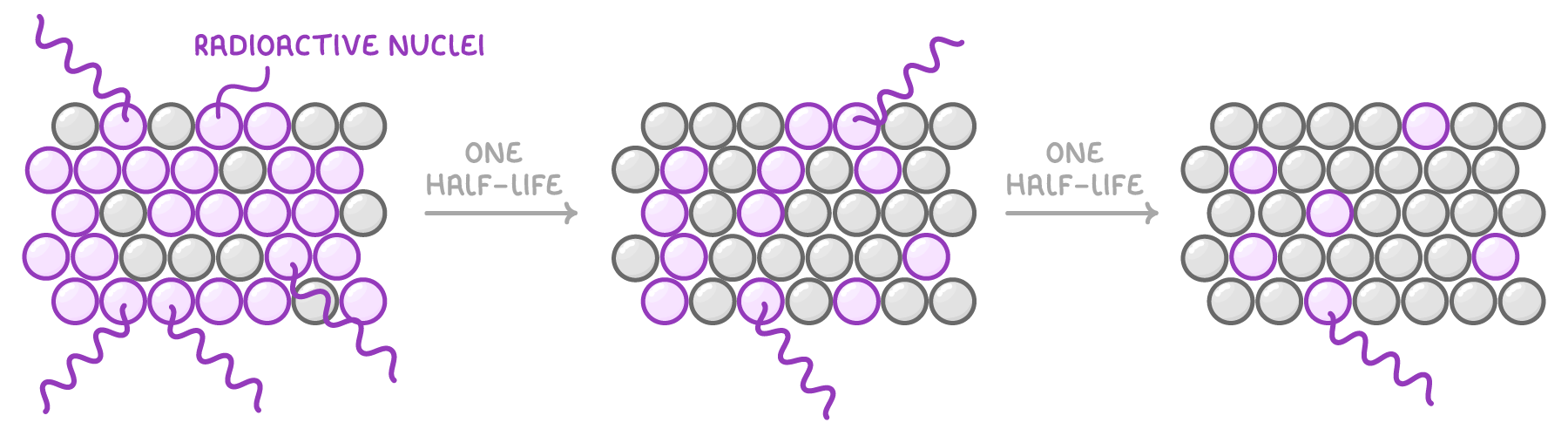
Purple nuclei are still radioactive; grey nuclei have already decayed.
Half-life and hazard
- Short half-life - Activity falls quickly: high radiation at the start, but the source soon becomes safe.
- Long half-life - Activity falls slowly: smaller amounts of radiation released, but for a very long time, so nearby areas stay exposed.
Finding half-life from a decay graph
A graph of activity (or count-rate, or number of radioactive nuclei) against time curves downwards, becoming less steep as time goes on.
Reading the half-life off the curve
- Read the initial value off the vertical axis.
- Work out half of this value.
- Find the time on the horizontal axis at which the curve reaches that halved value - that time is one half-life.
- Check by halving again: each successive halving should take the same length of time.
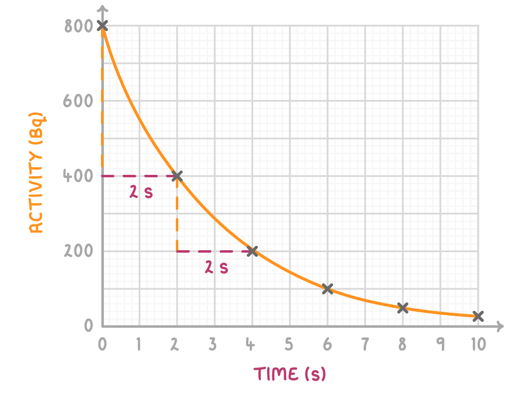
Subtract the background count first
- Before plotting, subtract the background count from every reading.
- If it isn't removed, the calculated half-life will be incorrect.
Worked example - Projecting activity forward
A sample of a radioactive isotope has an activity of 800 Bq and a half-life of 6 years. Find its activity after 12 years, and the net decline over that time.
Step 1 - Work forward one half-life at a time
After 1 half-life (6 years): 800 Bq ÷ 2 = 400 Bq
After 2 half-lives (12 years): 400 Bq ÷ 2 = 200 Bq
Step 2 - Find the net decline
The net decline compares the activity at the end of the period with the activity at the start.
Over 12 years it falls from 800 Bq to 200 Bq, a drop of 800 − 200 = 600 Bq.
As a ratio of the final activity to the original activity: 200 : 800 = 1 : 4. After two half-lives the activity has fallen to of its original value, a drop of .
Worked example - Time to reach a fraction of activity
The half-life of a radioactive sample is 90 minutes. How long does it take for the activity to fall to one quarter of its initial value?
Step 1 - Count the half-lives needed
full → one half → one quarter
That's two halvings, so two half-lives are needed.
Step 2 - Multiply by the half-life
Time = 2 × 90 minutes = 180 minutes (3 hours)