Half-Life definition

The half-life (t${}_{\frac{1}{2}}$) of a radioactive isotope is the time taken for half of the unstable nuclei in a sample to decay. Specifically, it is the time required for the number of undecayed nuclei to reduce to half its original value.

Longer half-lives indicate the isotope remains radioactive for longer periods. Shorter half-lives mean faster decay.

Exponential decay

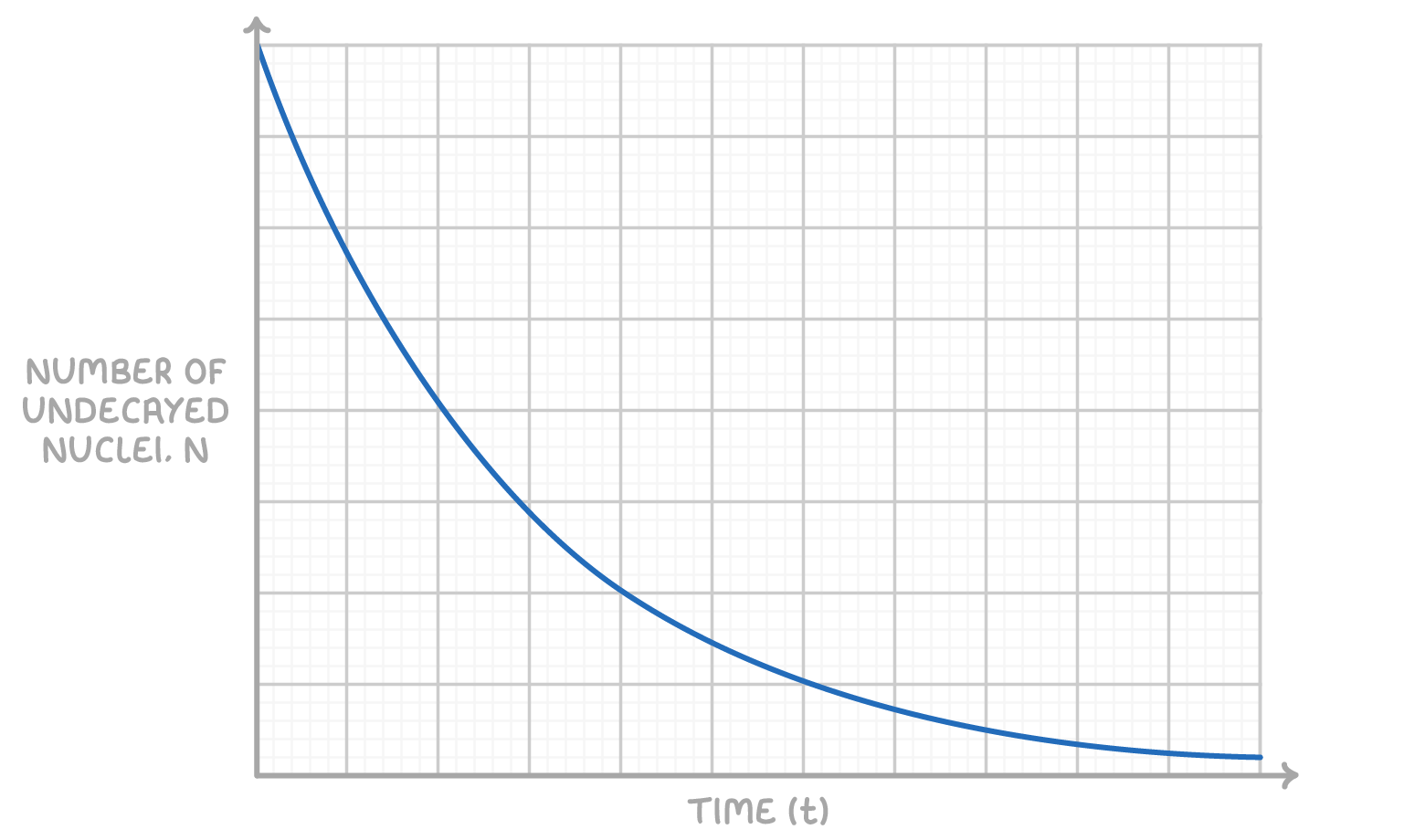
The decay of radioactive isotopes over time follows an exponential pattern. This makes the exact decay time of individual nuclei unpredictable.

However, the overall rate of decay for a large number of nuclei is predictable using probability statistics. This allows us to plot graphs showing the reduction in the number of undecayed nuclei over time.

Using decay graphs to determine half-life

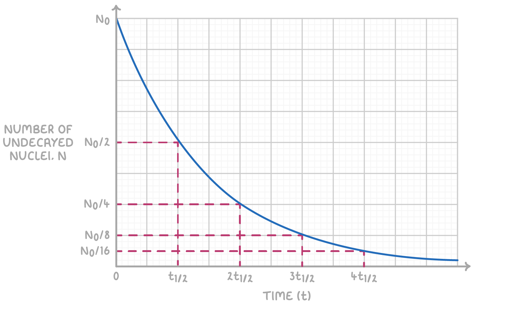
The half-life (t${}_{\frac{1}{2}}$) can be determined from exponential decay graphs in the following way:

1. Note the initial number of undecayed nuclei (N₀) when time t = 0
2. Locate the point on the curve corresponding to half of N0
3. Draw a line from the point to the time axis
4. The half-life is the time value where this intersects the axis

Experimentally generating count rate decay graphs

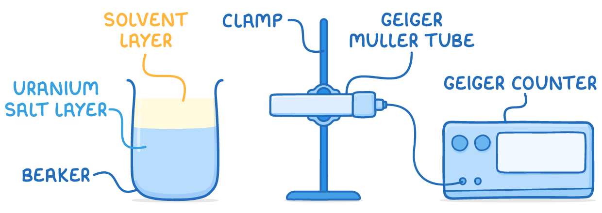
A common experiment involves using uranium salts to produce protactinium-234, then measuring its decay count rate over time.

Method:

1. Mix uranium salt with solvents then wait for layer separation
2. Position Geiger counter to detect decays from top solvent layer
3. Record count rate continuously from time of separation
4. Plot count rate values against time to obtain decay graph
5. Use decay graph to determine half-life as count rate reduces